When the Graph plotter starts, you will see the Edit data tab. Data can be entered, manipulated and saved in this view. The View graph tab is where the graphs are plotted.

• Working with the data table
• Importing:
  • tables
  • data
• Data separator
• Data format
• Assigning data to graph axes

• Graph display options
• Capturing the graph as a screenshot image
• Statistical output

Data can be entered, manipulated and saved in this view. Initially, the data table shows columns A and B with column A containing a list of integers. You do not have to complete all of the rows in the table in order to plot a graph.

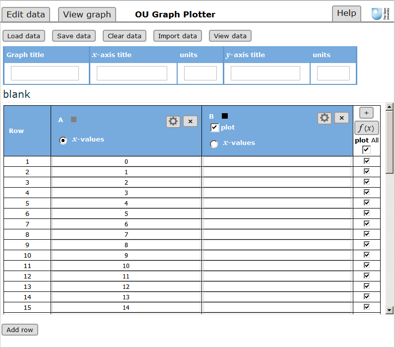
Figure 1 The Edit data view.

To enter or edit the title, axis labels or units for the graph, click or tap on the appropriate box in the small table above the main data table. Text can be formatted using the bold, italic, subscript and superscript buttons. (To remove the formatting, click on the box and edit the text manually.) Greek letters and the thermodynamic standard symbol are available from the symbols... drop-down list.

You may either enter a set of data into the table from scratch, or open an existing data set and make changes to it. The Load data button enables you to open stored data sets. To save a data set, use the Save data button. To clear the current data table, press the Clear data button.

To enter data into a table cell, click on the cell you wish to edit. Enter a value or modify an existing value using the keyboard.

To assist with data manipulation, there are a number of features available:

• The column data options button opens a box with the following:

  • Editing name / adding mathematecial functions

      Label name input (if it is inputted data) or Edit function button (if it is calculated data).
  • Marker shape or Color selections.
  • The Delete column button to delete the column from the table.
    

  • Importing a column of data

      Data for the column being edited can be imported using the Import column data button
      (if the column contains inputted data rather than calculated data).
    
    

    A text input box is provided to paste a list of numbers or radio buttons can be used to insert the following automatically calculated data: A list of numbers increasing by a fixed step A list of random numbers with a flat distribution between 0 and 1 A list of random numbers with a Gaussian distribution Columns with this data can then be added together with user defined functions from the calculator to produce a very wide variety of data points.

• The delete (×) button to delete the column from the table.
• The Add column (+) button adds a new column to the table to the right of existing columns. Thus, if columns A and B are present, pressing this button will create an empty column C.
• The f(x) button launches a calculator, which enables you to carry out mathematical operations on an existing column of data.
• The Add row button adds a new row to the data table.
• In the plot column, the checkbox for each row can be unchecked to omit a row from the plotted graph and/or the All checkbox can also be used.

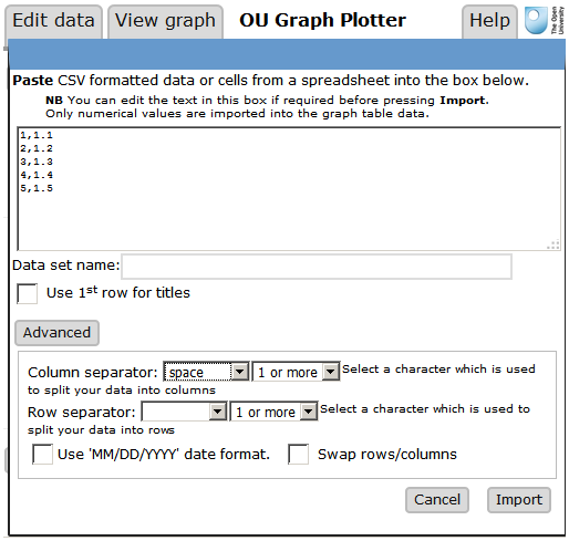
You can import data from other packages or text files by pressing the Import data button. The figures below show data imported from some selected and copied spreadsheet data cells.
Individual columns of data can also be imported using the column options button described above.

Figure 2 Using the Import data function.

The advanced button options enable you to adjust your imported data before it is imported into the Graph plotter table.

Data is imported into the graph plotter table as 'comma delimited'. Data pasted from different sources maybe separated by multiple tabs or spaces, so the Column separator can be used to convert your pasted data into the comma separated/delimited format.
Examples of typical pasted data and the result are shown below:

Example of pasted data
'tabbed' data from a spreadsheet: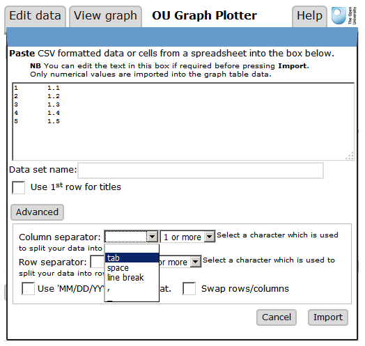	'spaced' data from a text file: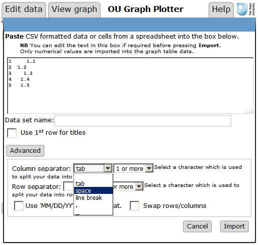
Result

N.B. Data in the x-values column can be entered as in a date format (DD/MM/YYYY and DD/MM/YY).

Data can be entered into the table in decimal format or using 'E' notation. Lower-case and upper-case e are accepted. Examples of valid number inputs are 0.00475, .6019, 432.87, 5.6e9, 1e-5, 4.3E10. It is not possible to enter numbers in scientific notation of the type 3.65 × 10^–9.

When you are ready to plot the data, use the radio buttons to specify which column to use for the horizontal x-values. Use the checkboxes to specify which column or columns to plot on the vertical y-axis. Press View graph to plot the graph and view it. The graph will be shown.

If the plot was successful, you will see the data points plotted on the graph and the numbers on the axes. Figure 2 shows a smooth curve fitted to a dataset. A tangent is drawn by clicking or tapping on the curve. Note that Graph plotter may format large or small values in your data to give compact numbers on the axes. To do this, it puts powers of 10 in the axis label. For example, 200 m may appear as 2 on the axis with 10² m in the axis label.

Figure 3 An example graph, showing a smooth curve and tangent.

The best way to capture a graph as an image file is by using a screen grabbing utility. Windows users may wish to use the 'Snipping Tool' which is either part of the operating system or can be downloaded. There are similar utilities available for Apple Macintosh computers. The resulting image can be inserted into a document or annotated with a graphics package. Make sure to save the data for the graph so that you may return to it later if necessary.

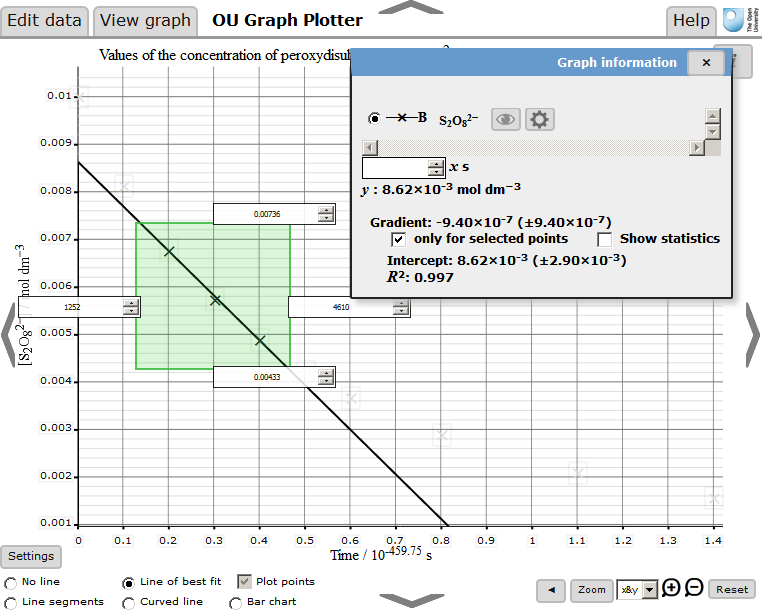
Straight line
On fitting a least squares best-fit line, you will see statistics for the line displayed in a box. The gradient and intercept are quoted, together with their associated uncertainties. Clicking or tapping on the graph will give you a readout of the x and y values at the current position. Keyboard users may enter a value in the box labelled 'x :' to achieve the same result.

You may also select an area of the graph by clicking and dragging to select particular points on the graph. You may also edit the numbers in the number boxes to fine adjust the dimensions of the green select area.
You can use the zoom functions and then re-adjust the selection area to further fine-tune the points used in the statistics calculations.

By checking 'only for selected points' the best fit line is calculated only using your selected points:


Curved line
The gradient (or slope) of a curved line at any point can be measured by clicking or tapping on the curve. The gradient at the chosen point appears in the box. Keyboard users may enter a value in the box labelled 'x :' to achieve the same result.

The calculator enables you to carry out mathematical operations on a column of data from the table. A new column in the data table will be created when you have successfully performed a calculation. The results in each cell need to be in terms of an existing column or columns. Cell numbers are displayed to upto 15 decimal places and in a lighter color to indicate that they cannot be edited.

By way of example, to calculate a new column C by taking the natural logarithm of each column B value, press the 'ln' button followed by the button labelled 'B'. The text ln(B) is inserted into the input box. Press Calculate, and the new column C is created in the table with the calculated values.

Figure 4 The Calculator window.

• The < and > buttons move the text input cursor. Text entries can be undone or cleared using the repsective buttons. It is generally recommended that you use the buttons to enter functions.
• The Exp button represents scientific notation. Thus, 1.2E9 is equivalent to 1.2 × 10⁹.
• The e button corresponds to Euler's number e (2.71828...).
• The exp button represents e^x. Thus, exp(2π) is equivalent to e^2π.
• The ^ button represents a value raised to a power. Thus, B^2 would square all the values in column B.
• The ln and log₁₀ buttons give logarithm to base e (natural logarithm) and logarithm to base 10, respectively.
• The abs button corresponds to the absolute value (or magnitude) of a real number, regardless of its sign.
• The sqrt button corresponds to the square root of a real number.
• The 1/x button corresponds to the reciprocal of the following real number.
• The sine, cosine and tangent (sin, cos, tan) functions are accompanied by their inverse functions asin, acos and atan.

The calculator operates in radians mode. Thus, to obtain cos 45°, you should enter cos(π/4).